Chapter 6 Country effects — fixed effects and multilevel modeling
Nested survey data call for explicit country handling. This chapter shows two approaches:
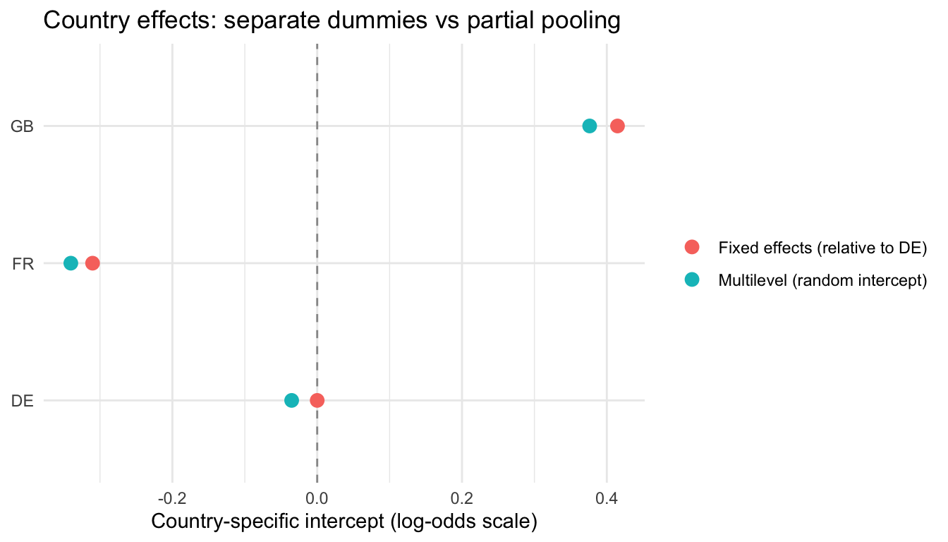
- Country fixed effects (dummies): absorbs unobserved, time-invariant differences between GB, DE, and FR.
- Multilevel (random-intercept) logistic regression: partially pools country effects, reducing noise for small samples and enabling variance decomposition.
A caveat before we start. This subset has only three level-2 units (countries). That is far below the usual guidance for multilevel models (roughly 20–30+ groups), so the estimated country-level variance and ICC below are unstable and should be read as a demonstration of the machinery, not as defensible estimates. With three groups, country fixed effects are the more honest choice; the multilevel results are included to illustrate partial pooling and shrinkage.
library(dplyr)
library(ggplot2)
library(broom)
library(broom.mixed)
library(lme4)
library(tidyr)

source("R/clean_ess.R")
source("R/theme_recsm.R")

ess <- clean_ess()
6.1 1. Country fixed effects (logit with dummies)
- Model:
news_regular ~ agea + gender + eduyrs + country - Interpretation: Country coefficients capture average gaps relative to the reference country (DE, alphabetically first).
fe_logit <- glm(news_regular ~ agea + gender + eduyrs + country,
                data = ess, family = binomial())
fe_tidy <- broom::tidy(fe_logit, exponentiate = TRUE, conf.int = TRUE)
6.1.0.1 Odds ratios
6.1.0.1.1 Table
## # A tibble: 6 x 7
##   term        estimate std.error statistic  p.value conf.low conf.high
##   <chr>          <dbl>     <dbl>     <dbl>    <dbl>    <dbl>     <dbl>
## 1 (Intercept)  0.00997  0.0971      -47.5  0         0.00824    0.0121
## 2 agea         1.04     0.000998     38.4  0         1.04       1.04
## 3 genderMale   1.47     0.0334       11.5  1.57e-30  1.37       1.57
## 4 eduyrs       1.03     0.00449       7.55 4.36e-14  1.03       1.04
## 5 countryFR    0.733    0.0460       -6.75 1.49e-11  0.670      0.802
## 6 countryGB    1.51     0.0370       11.2  3.56e-29  1.41       1.63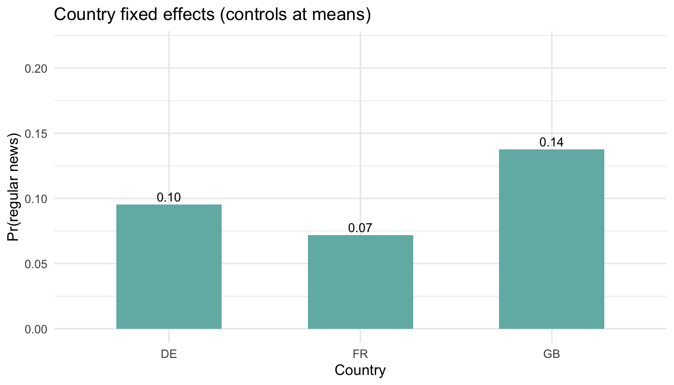
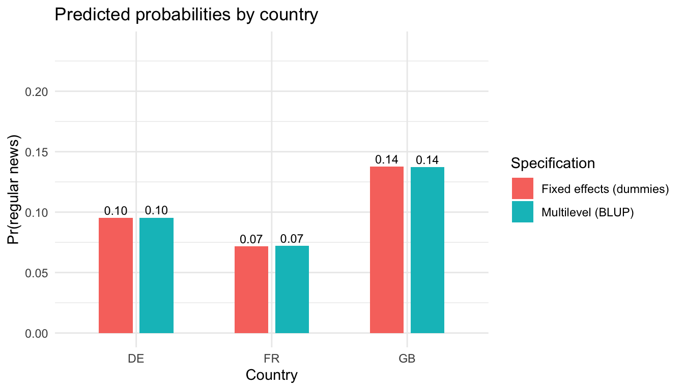
6.2 2. Multilevel logistic model (random intercepts by country)
- Model:
news_regular ~ agea + gender + eduyrs + (1 | country) - Why: Partial pooling shrinks extreme country estimates toward the grand mean, improving out-of-sample stability.
ml_logit <- glmer(news_regular ~ agea + gender + eduyrs + (1 | country),
                  data = ess, family = binomial(),
                  control = glmerControl(optimizer = "bobyqa"))

var_u0 <- as.numeric(VarCorr(ml_logit)$country)
icc <- var_u0 / (var_u0 + pi^2 / 3)
Intraclass correlation (ICC): 2.58% of the variance in the log-odds of regular news use is at the country level.
6.3 3. Random slopes for gender (optional extension)
With more countries, we could allow the gender gap to vary by country:
ml_logit_gender <- glmer(
  news_regular ~ agea + gender + eduyrs + (1 + gender | country),
  data = ess, family = binomial(),
  control = glmerControl(optimizer = "bobyqa")
)
In the current three-country sample this model may be over-parameterized; the random-intercept specification above is the stable classroom default.
6.4 Practice prompts
- Add an urban fixed effect to both models. Do city–rural gaps widen or narrow once country pooling is applied?
- Refit the multilevel model with
news_regulardefined as daily readership (nwsptot >= 5). How does the ICC change? - Replace
ageawith a spline (splines::ns(agea, df = 3)) inside both models and compare the resulting age profiles by country.