Chapter 7 Survey weighting — why and how
Survey data are collected with unequal selection probabilities. Inference should reflect the design to avoid biased point estimates and standard errors.
- Notation: Let \(w_i = 1/\pi_i\) be the design (inverse-probability) weight. For a finite population mean \(\bar{Y} = \sum_i w_i Y_i / \sum_i w_i\). For regression, weighted likelihoods re-scale each case by \(w_i\).
- ESS fields used:
pweight(post-stratification weight),psu(primary sampling unit),stratum(strata). We setoptions(survey.lonely.psu = "adjust")to stabilize single-PSU strata.
7.0.1 What these design variables mean (plain language)
pweight(post-stratification weight): Adjusts for unequal inclusion probabilities and aligns the achieved sample with known population margins (e.g., age × gender × region). Largepweightvalues upweight under-represented respondents; small values downweight over-represented ones.psu(primary sampling unit): The first cluster stage of selection (e.g., municipalities or postcode sectors). Respondents inside the same PSU share fieldwork and selection features, so their responses are correlated.stratum(strata): Mutually exclusive groups within which PSUs were sampled (e.g., by region × urbanicity). Stratification improves precision; variance estimation must respect it.- Design degrees of freedom: With clustering and stratification, the effective df are closer to the number of PSUs minus strata, not the raw respondent count—hence the importance of design-aware SEs.
library(dplyr)
library(ggplot2)
library(tidyr)
library(survey)
library(broom)

source("R/theme_recsm.R")

# Synthetic microdata to illustrate weighting without depending on raw ESS file quirks
set.seed(42)
n_psu <- 120
n_by_psu <- sample(8:18, n_psu, replace = TRUE)

demo_psu <- tibble(
  psu = 1:n_psu,
  stratum = sample(1:20, n_psu, replace = TRUE),
  country = sample(c("GB", "DE", "FR"), n_psu, replace = TRUE, prob = c(.4, .35, .25)),
  pweight = runif(n_psu, 0.5, 3),
  n = n_by_psu
)

ess_w <- demo_psu |>
  uncount(n) |>
  mutate(
    agea = pmin(pmax(round(rnorm(n(), 50, 15)), 18), 90),
    gender = sample(c("Male", "Female"), n(), replace = TRUE),
    # Generate outcome with country- and age-dependent probability
    linpred = -1 + 0.6 * (country == "GB") + 0.3 * (country == "FR") +
              0.01 * (agea - 50) + 0.4 * (gender == "Female"),
    news_regular = rbinom(n(), 1, plogis(linpred))
  ) |>
  select(psu, stratum, country, pweight, agea, gender, news_regular) |>
  mutate(country = factor(country),
         gender = factor(gender))

options(survey.lonely.psu = "adjust")
des <- svydesign(ids = ~psu, strata = ~stratum, weights = ~pweight,
                 data = ess_w, nest = TRUE)

svy_n <- nrow(des$variables)
7.1 1. Weighted descriptive estimates
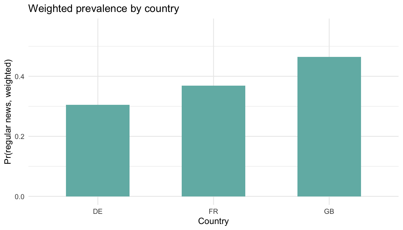
Respondents in the synthetic design: 1556.
##                 mean     SE
## news_regular 0.38522 0.0153- The point estimate is the design-weighted mean; SEs account for clustering and stratification.
- Design effect (
svymean(..., deff=TRUE)) tells how much variance inflation comes from the design versus SRS.
7.2 2. Weighted regression: linear probability and logit
lpm_w <- svyglm(news_regular ~ agea + gender + country,
                design = des, family = gaussian())
tidy(lpm_w)
## # A tibble: 5 x 5
## term estimate std.error statistic p.value
## <chr> <dbl> <dbl> <dbl> <dbl>
## 1 (Intercept) 0.234 0.0499 4.70 0.00000860
## 2 agea 0.00224 0.000799 2.80 0.00610
## 3 genderMale -0.0876 0.0243 -3.61 0.000497
## 4 countryFR 0.0681 0.0390 1.74 0.0844
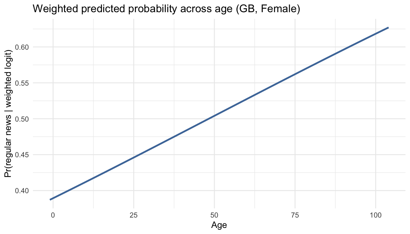
## 5 countryGB 0.155 0.0276 5.61 0.000000193logit_w <- svyglm(news_regular ~ agea + gender + country,
design = des, family = quasibinomial())
tidy(logit_w, exponentiate = TRUE)## # A tibble: 5 x 5
## term estimate std.error statistic p.value
## <chr> <dbl> <dbl> <dbl> <dbl>
## 1 (Intercept) 0.319 0.224 -5.11 0.00000165
## 2 agea 1.01 0.00353 2.77 0.00681
## 3 genderMale 0.682 0.105 -3.64 0.000434
## 4 countryFR 1.36 0.174 1.77 0.0807
## 5 countryGB 1.95 0.122 5.49 0.000000333Comparison points for students:
- Weights + clustering:
svyglmgives design-consistent SEs; plainglmdoes not. - Quasibinomial keeps logit link but uses robust variance; estimates mirror survey-weighted MLE when weights are scaled.
- LPM vs logit under weights: LPM slopes stay probability-difference interpretation; logit ORs remain multiplicative.
7.3 3. When to weight (practical guidance)
- Use design/post-strat weights when estimating population levels (means, totals, prevalence) or effects that might shift with differential selection.
- In randomized experiments or when modeling causal effects with ignorable sampling, weights may be optional; still cluster-robust SEs matter.
- If the research question is sample-only prediction, weights can be skipped, but report that scope-of-inference is limited.
7.5 Practice prompts
- Re-estimate the weighted mean of
news_regularand the country gaps without the design (a plainglm/weighted.meanignoringpsuandstratum). How do the point estimates and especially the standard errors move once the design is ignored? - Add the
gender × countryinteraction to the weighted logit. Do the country contrasts shift once the gap is allowed to vary by gender? - Estimate a design effect for
news_regular(svymean(~news_regular, des, deff = TRUE)) and discuss how many “effective” observations the clustered design corresponds to.
When you move to the real ESS file, the analogous extensions are to swap
pweightforanweightand to addeduyrs; the synthetic dataset here intentionally omits those columns.
Course assistant
Searches the book — no answers are made up