Chapter 3 Day 1 — Describing the ESS sample
Goal: practice measurement levels, univariate summaries, and basic visualisations using the ESS subset (GB, DE, FR).
3.1 Variables we use
ppltrst(0–10): generalised social trust (higher = more trust)agea: age in yearsgndr: 1 = male, 2 = female (other codes = missing)nwsptot: days per week reading newspapers (0–7; 66/77/88/99 = missing)netustm: minutes per day on the internetdomicil: 1 big city … 5 farm/countrysidecntry: GB, DE, FR
3.2 Measurement checks
ppltrstandagea: interval/ratio (mean and sd are fine).nwsptot,netustm: count-like; treat as interval for summaries but plot distributions.domicil: ordered categorical (use medians/percentiles).gndr: binary factor.
3.3 From description to inference
- Descriptive vs causal inference: describing “what is” (population levels, group gaps) vs “why” (causal claims require design/identification). Today we stay descriptive but prep for causal thinking.
- Sampling model: estimates come from a sample → always uncertainty. Sampling distributions tell us how much an estimator would vary across repeated samples.
- CLT intuition: for many statistics (like the mean), repeated samples stack up in an approximately normal bell curve as n grows; this justifies SEs, CIs, and t-tests.
- Hypothesis testing basics: state H0/HA, pick a test statistic, get a p-value, draw a conclusion while minding Type I (false positive) and Type II (false negative) risks.
3.4 Distributions and where centre matters
- Central tendency: use mean for roughly symmetric interval data (e.g.,
ppltrst), median for skewed or count-like data (e.g.,nwsptot), and mode/proportions for categorical (gndr,domicil). - Shapes to look for: symmetry vs. skew, heavy tails, spikes at 0, and multimodality. Use density/Histogram to diagnose before choosing a summary.
- Robustness: median and IQR resist outliers; mean and SD are more efficient when the distribution is near normal.
3.4.1 Quick distribution gallery
3.4.1.1 Code
ess <- clean_ess()
hist_trust <- ggplot(ess, aes(x = ppltrst)) +
geom_histogram(binwidth = 1, boundary = -0.5, fill = "#4C78A8") +
labs(title = "Generalised social trust", x = "Trust (0-10)", y = "Count") +
theme_recsm()
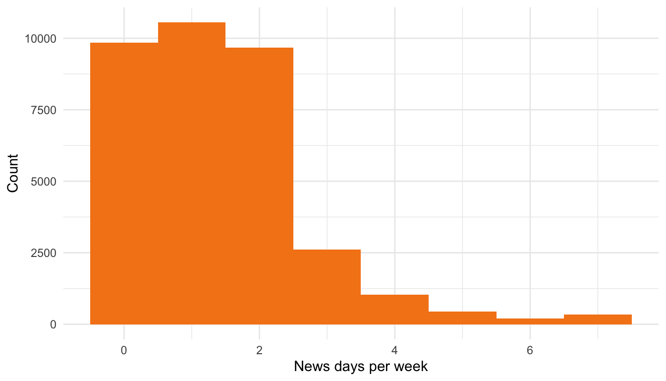
hist_news <- ggplot(ess, aes(x = nwsptot)) +
geom_histogram(binwidth = 1, fill = "#E69F00") +
labs(title = "Days per week reading news", x = "News days/week", y = "Count") +
theme_recsm()
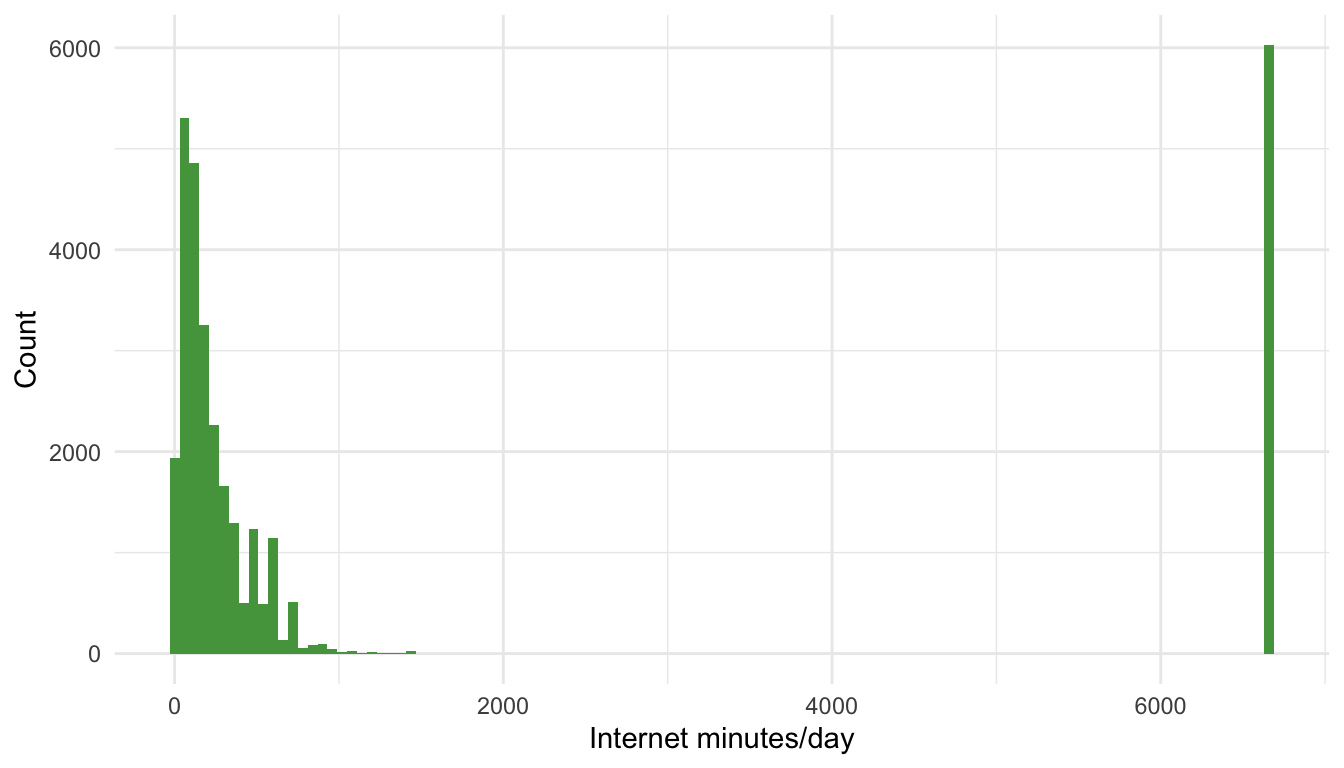
hist_net <- ggplot(ess, aes(x = netustm)) +
geom_histogram(binwidth = 60, boundary = 0, fill = "#009E73") +
labs(title = "Internet use on a typical day", x = "Internet minutes/day", y = "Count") +
theme_recsm()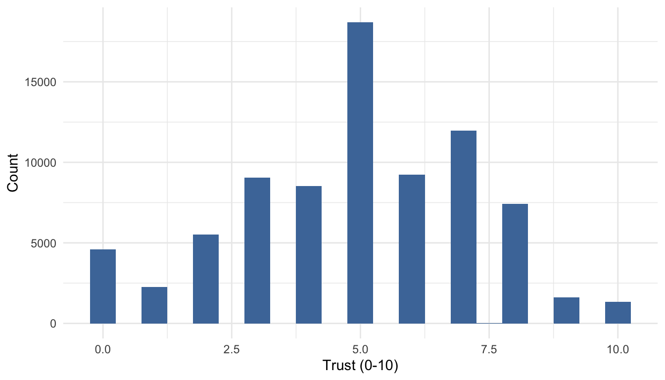
3.5 Problem set A — Univariate summaries
- Compute mean, median, variance, and IQR for
ppltrst,nwsptot, andnetustmfor each country. - Plot histograms (or density plots) of
ppltrstby country; compare centres and spread. - Produce a table of counts and proportions for
gndranddomicilby country.
3.5.1 Worked example A
3.5.1.1 Code
# code only (not executed in this tab)
summary_tbl <- ess |>
  group_by(cntry) |>
  summarise(
    trust_mean = mean(ppltrst, na.rm = TRUE),
    trust_sd   = sd(ppltrst, na.rm = TRUE),
    news_med   = median(nwsptot, na.rm = TRUE),
    news_iqr   = IQR(nwsptot, na.rm = TRUE),
    net_mean   = mean(netustm, na.rm = TRUE),
    net_sd     = sd(netustm, na.rm = TRUE)
  )

trust_plot <- ggplot(ess, aes(x = ppltrst, fill = cntry)) +
  geom_density(alpha = 0.35, adjust = 2.5, colour = NA) +
  labs(title = "Distribution of social trust by country",
       x = "Social trust (0-10)", y = "Density", fill = "Country") +
  theme_recsm()

counts <- ess |>
  mutate(dom_group = factor(domicil, levels = 1:5,
                            labels = c("Big city","Suburbs","Town","Village","Farm"))) |>
  count(cntry, gender, dom_group, name = "n") |>
  group_by(cntry) |>
  mutate(prop = n / sum(n))
3.5.1.2 Output
## # A tibble: 3 x 7
##   cntry trust_mean trust_sd news_med news_iqr net_mean net_sd
##   <chr>      <dbl>    <dbl>    <dbl>    <dbl>    <dbl>  <dbl>
## 1 DE          4.90     2.40        1        1     235.   204.
## 2 FR          4.53     2.18        1        2     196.   172.
## 3 GB          5.31     2.22        1        2     247.   203.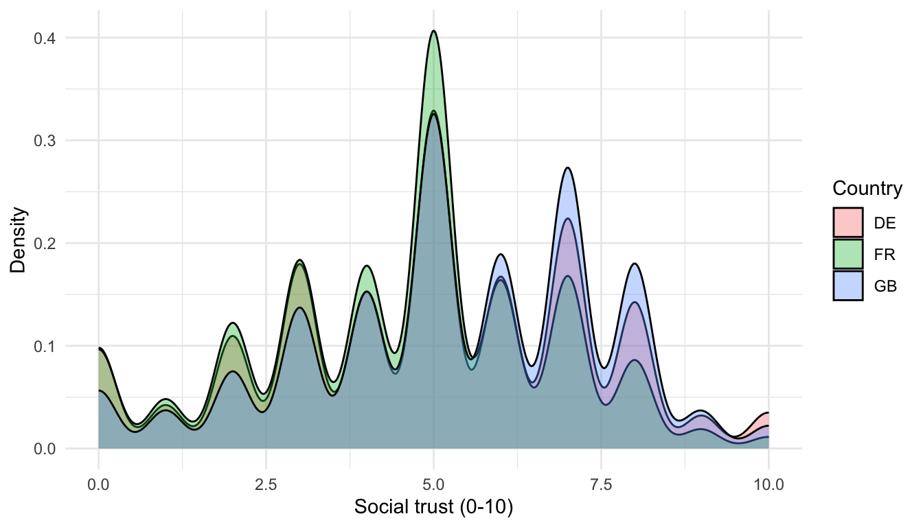
## # A tibble: 43 x 5
## # Groups:   cntry [3]
##    cntry gender dom_group     n    prop
##    <chr> <chr>  <fct>     <int>   <dbl>
##  1 DE    Female Big city   3212 0.0872
##  2 DE    Female Suburbs    2442 0.0663
##  3 DE    Female Town       6723 0.182
##  4 DE    Female Village    5354 0.145
##  5 DE    Female Farm        391 0.0106
##  6 DE    Female <NA>         86 0.00233
##  7 DE    Male   Big city   3144 0.0853
##  8 DE    Male   Suburbs    2396 0.0650
##  9 DE    Male   Town       6475 0.176
## 10 DE    Male   Village    5739 0.156
## # i 33 more rows
3.6 Problem set B — Bivariate exploration
- Correlate
ppltrstwithageaoverall and by country. Does trust rise or fall with age? - Create side-by-side boxplots of
ppltrstbygenderwithin each country. - Compute the difference in mean
ppltrstbetween genders; provide 95% confidence intervals using a t-test. - Produce a country-by-gender table of median
nwsptot.
3.6.1 Worked example B
3.6.1.1 Code
# code only (not executed in this tab)
cor_age_trust <- ess |>
  group_by(cntry) |>
  summarise(corr = cor(ppltrst, agea, use = "pairwise.complete.obs"))

boxplot_trust <- ggplot(filter(ess, !is.na(gender)), aes(x = gender, y = ppltrst, fill = gender)) +
  geom_boxplot(outlier.alpha = 0.2) +
  facet_wrap(~ cntry) +
  labs(x = NULL, y = "Social trust") +
  theme_recsm() +
  theme(legend.position = "none")

# difference in means with CI
trust_ttest <- t.test(ppltrst ~ gender, data = ess)
3.6.1.2 Output
## # A tibble: 3 x 2
##   cntry     corr
##   <chr>    <dbl>
## 1 DE     0.00129
## 2 FR    -0.0291
## 3 GB     0.0782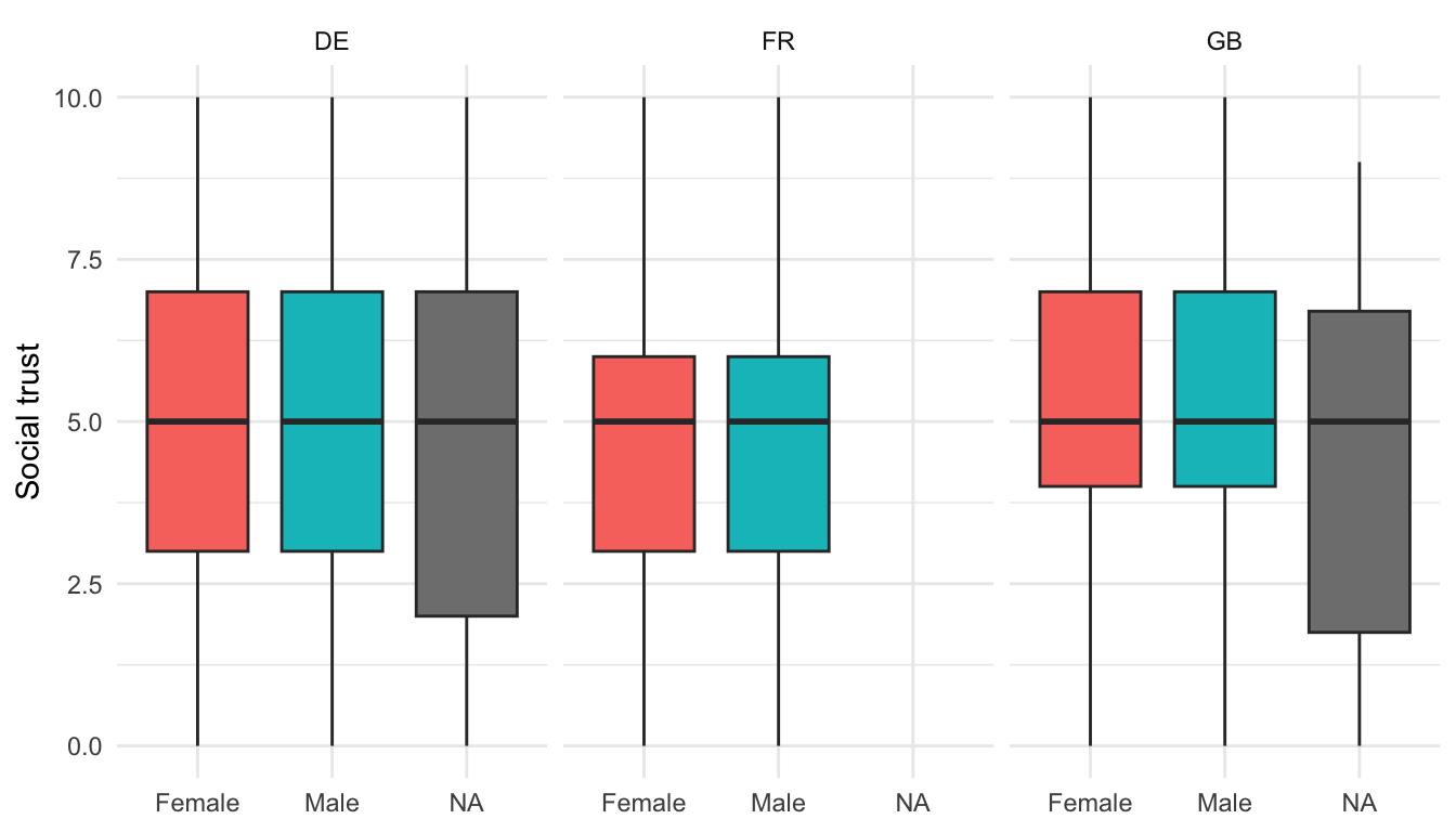
##
##  Welch Two Sample t-test
##
## data:  ppltrst by gender
## t = -6.3769, df = 79520, p-value = 1.817e-10
## alternative hypothesis: true difference in means between group Female and group Male is not equal to 0
## 95 percent confidence interval:
##  -0.13604975 -0.07207948
## sample estimates:
## mean in group Female   mean in group Male
##             4.870032             4.974096
3.7 Hypothesis testing quick-start
Two worked examples to introduce formal testing on Day 1.
3.7.1 Example 1: Two-sample t-test (mean trust by gender)
3.7.1.2 Output
##
##  Welch Two Sample t-test
##
## data:  ppltrst by gender
## t = -6.3769, df = 79520, p-value = 1.817e-10
## alternative hypothesis: true difference in means between group Female and group Male is not equal to 0
## 95 percent confidence interval:
##  -0.13604975 -0.07207948
## sample estimates:
## mean in group Female   mean in group Male
##             4.870032             4.974096
Interpretation: If the p-value < 0.05, we reject equal mean trust between men and women. The 95% CI shows the plausible range of the mean difference (Female − Male); if it excludes 0, the gap is statistically significant.
3.7.2 Example 2: Chi-squared test (gender × regular news readership)
3.7.2.2 Output
##
##              0     1
##   Female 16142  2086
##   Male   13917  2532
##
## Pearson's Chi-squared test with Yates' continuity correction
##
## data: tab_news
## X-squared = 116.47, df = 1, p-value < 2.2e-16Interpretation: A small p-value means the share of regular news readers differs by gender (variables not independent). Report the chi-squared statistic, degrees of freedom, and p-value.
3.8 Reflection prompts
- Which variables are most skewed? How does that affect your choice of centre and spread?
- Are gender gaps in trust consistent across GB, DE, and FR?
- If
nwsptothas many zeros, is median more informative than mean?
Use these as warm-ups before moving into regression modeling in the next chapter.
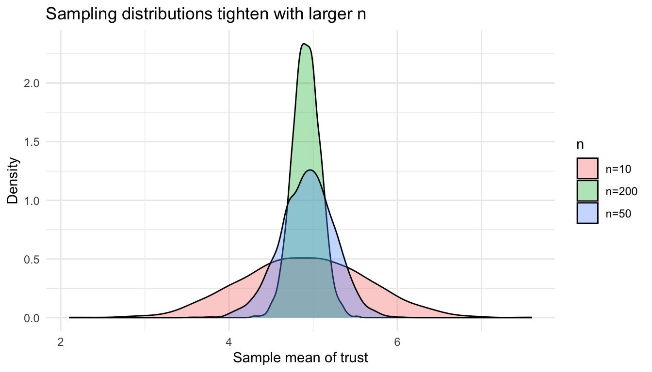
3.9 Sampling distributions by simulation
Central-limit intuition: as sample size grows, the sampling distribution of the mean tightens and approaches normality, even for skewed variables.
3.10 Hypothesis testing recap (slides → practice)
- T-tests compare means using the t distribution (fatter tails for small n); for two groups assume equal variances or use Welch when in doubt.
- Chi-squared tests independence in contingency tables.
- Errors: α = P(Type I), β = P(Type II); lowering α raises β. Report p-values and confidence intervals to show effect size and uncertainty.
- Confidence intervals: estimate ± (critical value × SE); if 95% CI excludes 0 (for mean differences), the two-sided test at α = 0.05 would reject H0.