Chapter 5 Day 3 — Non-linear models: logistic regression
We now model binary outcomes. This replaces the old factor-analysis/PCA content and links three specifications:
- Linear probability model (LPM): \(Y_i \in \{0,1\},\ \mathbb{E}[Y_i\mid X_i]=X_i\beta\) (identity link).
- Logit: \(p_i = \Pr(Y_i=1\mid X_i)=\operatorname{logit}^{-1}(X_i\beta)=\frac{e^{X_i\beta}}{1+e^{X_i\beta}}\).
- Marginal effects: \(\frac{\partial p_i}{\partial x_{ik}} = p_i(1-p_i)\beta_k\), highlighting how effects vary with the baseline probability.
- Interaction in logit: For \(p_i = \operatorname{logit}^{-1}(\eta_i)\) with \(\eta_i = \beta_0 + \beta_1 x + \beta_2 z + \beta_3 xz\), the general cross-partial effect is \(\frac{\partial^2 p_i}{\partial x\,\partial z} = p_i(1-p_i)(1-2p_i)(\beta_1+\beta_3 z)(\beta_2+\beta_3 x) + p_i(1-p_i)\beta_3\). Evaluated at \(x=z=0\) this reduces to \(p_i(1-p_i)(1-2p_i)\beta_1\beta_2 + p_i(1-p_i)\beta_3\). The key point: even the sign of the interaction effect can vary with \(p_i\), so it cannot be read off \(\beta_3\) alone (Ai & Norton, 2003).
Outcome: news_regular = 1 if a respondent reads newspapers on at least 3 days per week (nwsptot >= 3), 0 otherwise.
Predictors: age (agea), gender (gndr), country (cntry), education (eduyrs), and their interactions.
library(dplyr)
library(broom)
library(ggplot2)
library(marginaleffects)

source("R/clean_ess.R")
source("R/theme_recsm.R")

ess <- clean_ess()

# Fit once and reuse
lpm1   <- lm(news_regular ~ agea + gender + country, data = ess)
logit1 <- glm(news_regular ~ agea + gender + country, data = ess, family = binomial())
logit2 <- glm(news_regular ~ gender * country + agea, data = ess, family = binomial())
logit3 <- glm(news_regular ~ gender * agea + country + eduyrs, data = ess, family = binomial())
logit4 <- glm(news_regular ~ agea * eduyrs + gender + country, data = ess, family = binomial())
logit5 <- glm(news_regular ~ gender * agea * country + eduyrs, data = ess, family = binomial())

# Prediction data for plots
age_seq <- seq(min(ess$agea, na.rm = TRUE), max(ess$agea, na.rm = TRUE), length.out = 60)
edu_seq <- seq(min(ess$eduyrs, na.rm = TRUE), max(ess$eduyrs, na.rm = TRUE), length.out = 40)

nd2 <- expand.grid(country = c("GB","DE","FR"),
                   gender = c("Male","Female"),
                   agea = mean(ess$agea, na.rm = TRUE))
pred2 <- predict(logit2, newdata = nd2, type = "link", se.fit = TRUE)
nd2$pr <- plogis(pred2$fit)
nd2$lo <- plogis(pred2$fit - 1.96 * pred2$se.fit)
nd2$hi <- plogis(pred2$fit + 1.96 * pred2$se.fit)
plot_gender_country <- ggplot(nd2, aes(x = country, y = pr, fill = gender)) +
  geom_col(position = position_dodge(width = 0.6), width = 0.5) +
  geom_errorbar(aes(ymin = lo, ymax = hi), position = position_dodge(width = 0.6), width = 0.2) +
  labs(y = "Pr(regular news)") +
  theme_recsm()

nd3 <- expand.grid(agea = age_seq, gender = c("Male","Female"),
                   country = "GB", eduyrs = mean(ess$eduyrs, na.rm = TRUE))
pred3 <- predict(logit3, newdata = nd3, type = "link", se.fit = TRUE)
nd3$pr <- plogis(pred3$fit)
nd3$lo <- plogis(pred3$fit - 1.96 * pred3$se.fit)
nd3$hi <- plogis(pred3$fit + 1.96 * pred3$se.fit)
plot_gender_age <- ggplot(nd3, aes(x = agea, y = pr, color = gender)) +
  geom_line(linewidth = 1) +
  geom_ribbon(aes(ymin = lo, ymax = hi, fill = gender), alpha = 0.15, color = NA) +
  labs(y = "Pr(regular news)", x = "Age") +
  theme_recsm()

nd4 <- expand.grid(eduyrs = edu_seq,
                   agea = quantile(ess$agea, c(.2,.5,.8), na.rm = TRUE),
                   gender = "Male", country = "GB")
pred4 <- predict(logit4, newdata = nd4, type = "link", se.fit = TRUE)
nd4$pr <- plogis(pred4$fit)
nd4$lo <- plogis(pred4$fit - 1.96 * pred4$se.fit)
nd4$hi <- plogis(pred4$fit + 1.96 * pred4$se.fit)
plot_age_edu <- ggplot(nd4, aes(x = eduyrs, y = pr, color = factor(agea))) +
  geom_line(linewidth = 1) +
  geom_ribbon(aes(ymin = lo, ymax = hi, fill = factor(agea)), alpha = 0.12, color = NA) +
  labs(y = "Pr(regular news)", x = "Years of education", color = "Age quantile") +
  theme_recsm()

nd5 <- expand.grid(agea = age_seq,
                   gender = c("Male","Female"),
                   country = c("GB","DE","FR"),
                   eduyrs = mean(ess$eduyrs, na.rm = TRUE))
pred5 <- predict(logit5, newdata = nd5, type = "link", se.fit = TRUE)
nd5$pr <- plogis(pred5$fit)
nd5$lo <- plogis(pred5$fit - 1.96 * pred5$se.fit)
nd5$hi <- plogis(pred5$fit + 1.96 * pred5$se.fit)
plot_threeway <- ggplot(nd5, aes(x = agea, y = pr, color = gender)) +
  geom_line() +
  geom_ribbon(aes(ymin = lo, ymax = hi, fill = gender), alpha = 0.12, color = NA) +
  facet_wrap(~ country) +
  labs(y = "Pr(regular news)", x = "Age") +
  theme_recsm()

# Average marginal effects on the probability scale, with delta-method 95% CIs.
# agea = 1  -> average change in Pr(regular news) for one more year of age.
# gender    -> average Female - Male difference (c("Male","Female") sets the
#              baseline first, so the contrast is Pr(Female) - Pr(Male)).
ame_table <- avg_comparisons(
  logit5,
  variables = list(agea = 1, gender = c("Male", "Female"))
) |>
  dplyr::transmute(
    term, contrast,
    AME = estimate, conf.low, conf.high, p.value
  )

# How the Female - Male probability gap changes across age (95% CI ribbon),
# at typical education, averaged over countries. plot_comparisons builds the
# age grid and propagates uncertainty for us.
me_female_plot <- plot_comparisons(
  logit5,
  variables = list(gender = c("Male", "Female")),
  condition = "agea"
) +
  geom_hline(yintercept = 0, linetype = "dashed", colour = "grey55") +
  labs(
    x = "Age", y = "Pr(Female) - Pr(Male)",
    title = "Marginal effect of being Female on regular news reading",
    subtitle = "Difference in predicted probability across age, with 95% CI"
  ) +
  theme_recsm()
5.1 0. Linear probability model (LPM) first
- Specification: \(Y_i = X_i\beta + \varepsilon_i,\ Y_i \in \{0,1\}\). Ordinary least squares with a binary outcome.
- Pros: Coefficients are immediate probability changes (\(\Delta p\)) per unit of \(X\); easy to interpret and to add fixed effects.
- Cons: Predicted values can leave \([0,1]\); errors are heteroskedastic; marginal effects are assumed constant even when baseline risk is near 0 or 1.
- When is LPM “safe enough”? Middle-range probabilities (e.g., 0.2–0.8), modest leverage points, and when the goal is fast descriptive decomposition or fixed-effects absorption. Use robust standard errors.
library(sandwich)
library(lmtest)

lpm_vcov <- sandwich::vcovHC(lpm1, type = "HC1")
lpm_tidy <- broom::tidy(lpm1, conf.int = TRUE, vcov = lpm_vcov)
5.1.0.1 Output
## # A tibble: 5 x 7
##   term        estimate std.error statistic  p.value conf.low conf.high
##   <chr>          <dbl>     <dbl>     <dbl>    <dbl>    <dbl>     <dbl>
## 1 (Intercept) -0.0861  0.00569      -15.1  1.43e-51 -0.0973   -0.0750
## 2 agea         0.00397 0.0000969     40.9  0         0.00378   0.00416
## 3 genderMale   0.0429  0.00356       12.0  2.31e-33  0.0359    0.0498
## 4 countryFR   -0.0334  0.00442       -7.56 4.08e-14 -0.0421   -0.0248
## 5 countryGB    0.0490  0.00418       11.7  9.41e-32  0.0408    0.0572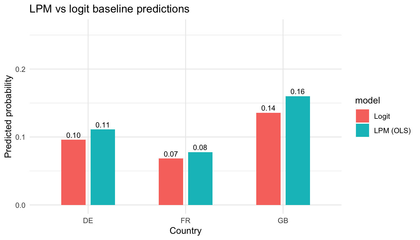
5.2 1. Simple logistic model
5.2.1 Simple logistic model
5.2.1.1 Code
logit1 <- glm(news_regular ~ agea + gender + country, data = ess, family = binomial())
broom::tidy(logit1, exponentiate = TRUE, conf.int = TRUE)
Odds ratios > 1 indicate higher odds of being a regular news reader.
5.2.1.2 Output
## # A tibble: 5 x 7
##   term        estimate std.error statistic  p.value conf.low conf.high
##   <chr>          <dbl>     <dbl>     <dbl>    <dbl>    <dbl>     <dbl>
## 1 (Intercept)   0.0175  0.0624      -64.9  0          0.0155    0.0197
## 2 agea          1.04    0.000941     38.5  0          1.04      1.04
## 3 genderMale    1.50    0.0330       12.2  3.33e-34   1.40      1.60
## 4 countryFR     0.692   0.0452       -8.16 3.34e-16   0.633     0.755
## 5 countryGB     1.48    0.0367       10.7  9.12e-27   1.38      1.59
Interpretation: Odds ratios >1 raise the chance of regular news use; check if the CI excludes 1 for age, gender, or specific countries before claiming significance.
5.3 2. Binary × Binary interaction (gender × country)
5.3.0.2 Output
## # A tibble: 7 x 7
## term estimate std.error statistic p.value conf.low conf.high
## <chr> <dbl> <dbl> <dbl> <dbl> <dbl> <dbl>
## 1 (Intercept) 0.0180 0.0662 -60.7 0 0.0158 0.0205
## 2 genderMale 1.41 0.0522 6.61 3.83e-11 1.27 1.56
## 3 countryFR 0.643 0.0673 -6.57 5.14e-11 0.563 0.733
## 4 countryGB 1.42 0.0536 6.55 5.87e-11 1.28 1.58
## 5 agea 1.04 0.000941 38.5 0 1.04 1.04
## 6 genderMale:countryFR 1.14 0.0907 1.47 1.42e- 1 0.957 1.37
## 7 genderMale:countryGB 1.08 0.0735 1.04 2.97e- 1 0.935 1.25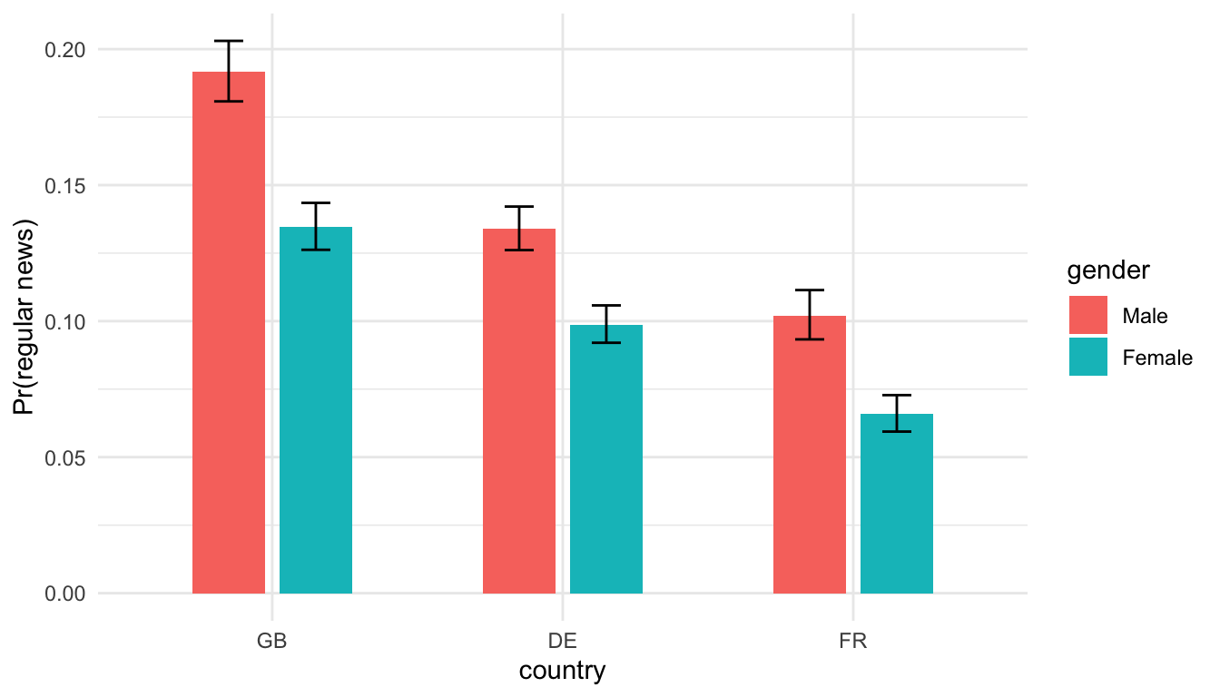 Interpretation: If male–female bars overlap within countries (CI bars), gender differences are modest. Compare across countries to see where the gap is largest.
5.4 3. Binary × Continuous interaction (gender × age)
5.4.0.2 Output
## # A tibble: 7 x 7
## term estimate std.error statistic p.value conf.low conf.high
## <chr> <dbl> <dbl> <dbl> <dbl> <dbl> <dbl>
## 1 (Intercept) 0.0109 0.114 -39.6 0 0.00868 0.0136
## 2 genderMale 1.26 0.113 2.03 4.22e- 2 1.01 1.57
## 3 agea 1.04 0.00141 26.2 1.61e-151 1.03 1.04
## 4 countryFR 0.733 0.0460 -6.76 1.34e- 11 0.669 0.802
## 5 countryGB 1.51 0.0370 11.2 3.74e- 29 1.41 1.63
## 6 eduyrs 1.03 0.00450 7.45 9.68e- 14 1.02 1.04
## 7 genderMale:agea 1.00 0.00192 1.41 1.58e- 1 0.999 1.01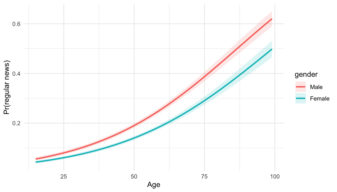 Interpretation: Diverging ribbons indicate age effects differ by gender; if both ribbons rise similarly, the interaction is weak.
5.5 4. Continuous × Continuous interaction (age × education)
5.5.0.2 Output
## # A tibble: 7 x 7
## term estimate std.error statistic p.value conf.low conf.high
## <chr> <dbl> <dbl> <dbl> <dbl> <dbl> <dbl>
## 1 (Intercept) 0.0133 0.223 -19.4 1.12e-83 0.00860 0.0206
## 2 agea 1.03 0.00353 9.47 2.80e-21 1.03 1.04
## 3 eduyrs 1.01 0.0162 0.707 4.80e- 1 0.980 1.04
## 4 genderMale 1.46 0.0334 11.4 6.41e-30 1.37 1.56
## 5 countryFR 0.737 0.0461 -6.63 3.29e-11 0.673 0.806
## 6 countryGB 1.52 0.0370 11.2 2.53e-29 1.41 1.63
## 7 agea:eduyrs 1.00 0.000270 1.44 1.50e- 1 1.00 1.00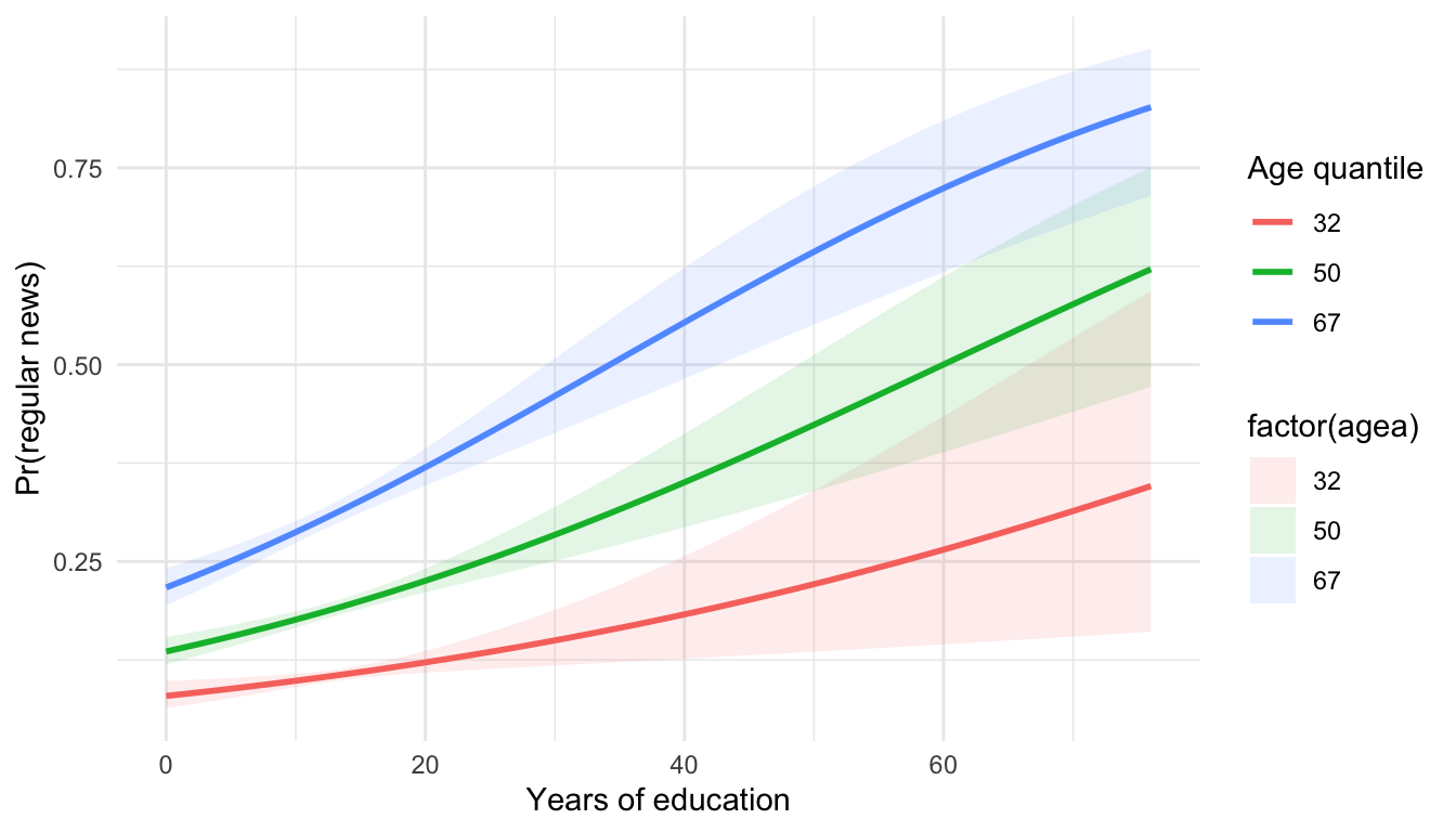 Interpretation: Steeper lines for higher age quantiles would mean education matters more (or less) for older respondents; overlap implies limited moderation.
5.6 5. Three-way interaction (gender × age × country)
5.6.0.2 Output
## # A tibble: 13 x 7
## term estimate std.error statistic p.value conf.low conf.high
## <chr> <dbl> <dbl> <dbl> <dbl> <dbl> <dbl>
## 1 (Intercept) 0.00660 0.164 -30.7 2.20e-206 0.00477 0.00907
## 2 genderMale 0.809 0.203 -1.04 2.97e- 1 0.543 1.20
## 3 agea 1.05 0.00240 19.3 6.67e- 83 1.04 1.05
## 4 countryFR 1.52 0.232 1.82 6.91e- 2 0.965 2.40
## 5 countryGB 3.30 0.187 6.38 1.73e- 10 2.29 4.76
## 6 eduyrs 1.03 0.00452 7.28 3.30e- 13 1.02 1.04
## 7 genderMale:agea 1.01 0.00336 2.79 5.33e- 3 1.00 1.02
## 8 genderMale:country~ 1.29 0.324 0.793 4.28e- 1 0.685 2.44
## 9 genderMale:country~ 2.46 0.260 3.46 5.37e- 4 1.48 4.10
## 10 agea:countryFR 0.986 0.00387 -3.66 2.57e- 4 0.979 0.993
## 11 agea:countryGB 0.986 0.00311 -4.69 2.77e- 6 0.980 0.992
## 12 genderMale:agea:co~ 0.998 0.00542 -0.400 6.89e- 1 0.987 1.01
## 13 genderMale:agea:co~ 0.985 0.00438 -3.34 8.46e- 4 0.977 0.994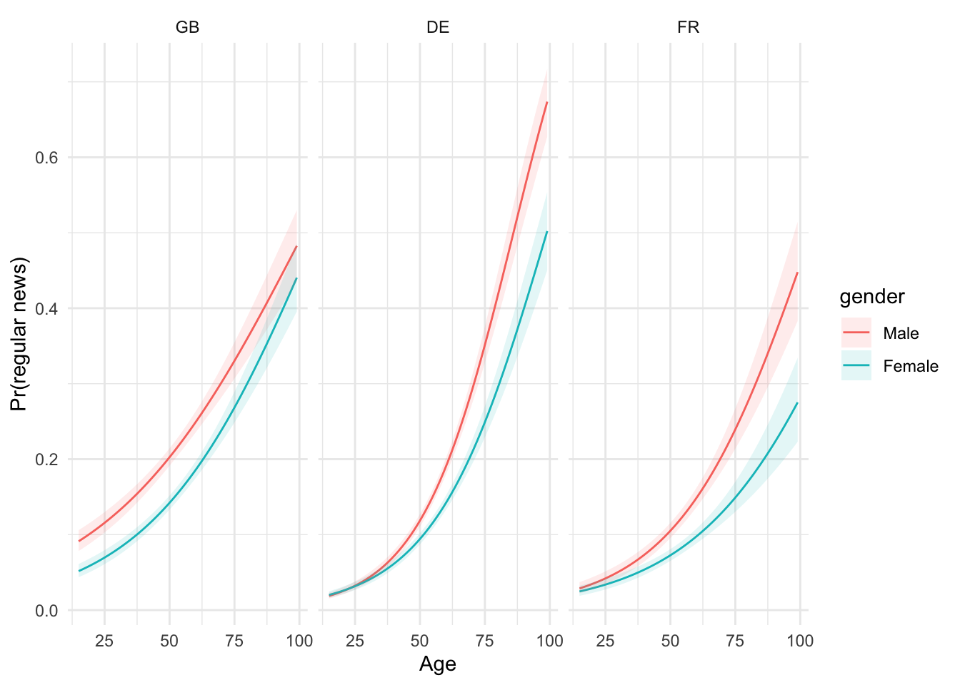 Interpretation: Scan each country facet—if ribbons separate widely, the age–gender pattern is country-specific; overlapping ribbons suggest similar patterns across countries.
5.7 6. Marginal effects and interpretation
library(marginaleffects)

# Average marginal effects on the probability scale (delta-method 95% CIs)
avg_comparisons(logit5, variables = list(agea = 1, gender = c("Male", "Female")))

# The Female - Male probability gap as a function of age, with a 95% ribbon
plot_comparisons(logit5, variables = list(gender = c("Male", "Female")),
condition = "agea")- Prefer predicted probabilities and marginal effects over raw log-odds.
- Read the ribbon, not just the point estimate: where it crosses zero, the gender gap is not distinguishable from no difference.
- Inspect separation or influential points with
performance::check_model(logit5)if desired.
5.7.1 AMEs and focal contrasts
5.7.1.1 Code
# Average marginal effects table (probability scale, 95% CIs)
ame_table <- avg_comparisons(
  logit5,
  variables = list(agea = 1, gender = c("Male", "Female"))
)

# Female - Male probability gap across age, with a 95% confidence ribbon
me_female_plot <- plot_comparisons(
  logit5,
  variables = list(gender = c("Male", "Female")),
  condition = "agea"
)
5.7.1.2 Output
##
##    Term      Contrast Pr(>|z|)   CI low  CI high
##  agea   +1              <0.001  0.00397  0.00439
##  gender Female - Male   <0.001 -0.04857 -0.03450
##
## Columns: term, contrast, AME, conf.low, conf.high, p.value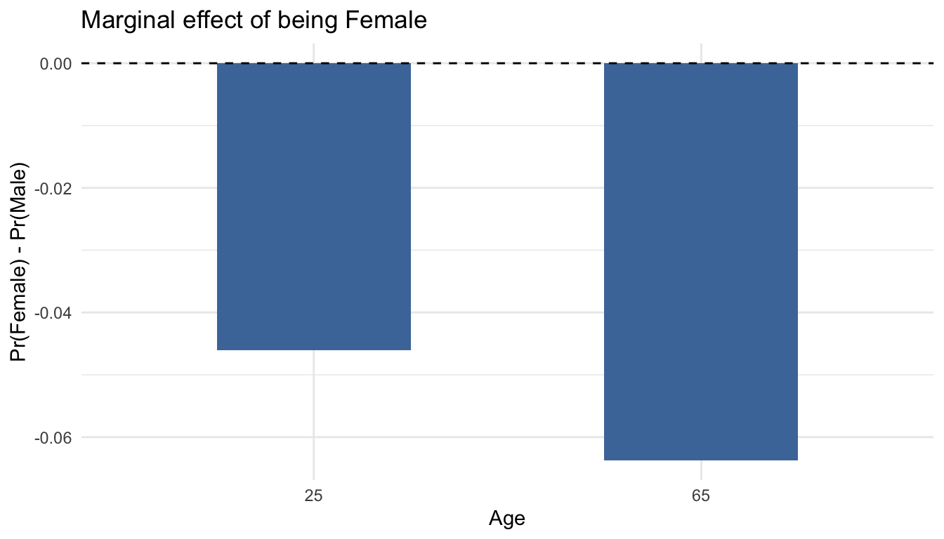
Interpretation: The table reports average marginal effects on the probability scale — the average change in the probability of regular news reading for one more year of age, and for being Female rather than Male — each with a 95% confidence interval. The curve shows how the Female − Male gap evolves across age: where the line sits above the dashed zero line, women are predicted to read regularly more often than men; where the shaded 95% band overlaps zero, that gap is not statistically distinguishable from no difference.
Country-level pooling choices (fixed vs multilevel) are expanded in the next chapter.
5.8 Problem set — Logistic regression practice
- Recode the outcome as
news_daily = nwsptot >= 5and re-estimatelogit3. How do the marginal effects of age change when the bar for “regular” consumption is higher? - Add
urban(1/2 = urban, 3–5 = non-urban) as a predictor and interact it withcountry. Which country shows the largest urban–rural gap in news readership? - Compare
logit4andlogit5using AIC and pseudo R² (pscl::pR2). Which balance of complexity and fit seems reasonable for classroom examples? - For one model, translate results into plain language for a non-technical audience: choose two profiles (e.g., 30-year-old woman in GB vs 60-year-old man in FR) and report predicted probabilities.
These exercises deliver a full set of interaction types in a nonlinear setting, ready to complement your lecture slides.